Hidden tricks in Excel functions and User interface

Today we are going to discuss about hidden abilities of excel functions and user interface techniques. We will see 3 tricks in each category of function and user interface.

Lot to learn, let's dive in.

Excel function:

Trick 1 - Month number from month name:

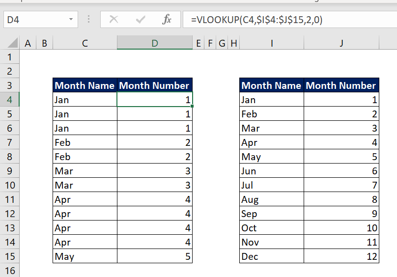
Consider that we have month name in our data, and we need to find month number.

In common practice, we do this in 2 ways.

1. Helper table with Month name and Month number and use VLOOKUP function.

2. Helper column with Month Name and use MATCH function.

Let me show you the glimpse of above 2 methods.

One more method is there, which will do this task with ease.

We can use MONTH function with bit of tweak to accomplish this task,

Argument of this function is,

=MONTH(serial_number)

If we feed date as serial number, then this function will deliver the month number of date.

Here we have only month name, if we feed month name into MONTH function, it will throw an error. But excel can understand the dates in text format. Let's see an example.

=MONTH("15-Sep") delivers 9 as output,

So, we are going to tweak our month name into text date format as shown below,

=MONTH(C4&0)

 We used joining operator ampersand to concatenate month name with zero. We can use any number from 0 to 9. Then it becomes,

 =MONTH("Jan0")

Month number of this date in text format is 1. Simple but powerful.

Trick 2 - Extract quarter from date:

There are 2 ways to accomplish this task.

Method 1: combination of INT and MONTH.

Formula in D4 cell is,

=INT((MONTH(C4)-1)/3)+1

MONTH function delivers the month number of date 15/03/2024, which is 3.

Subtract 1 to get the nearest smaller integer. Since, we have 3 months in every quarter, we divide it by 3. Interim result till this point is 0.66667, if we wrap this value in INT function, then the result is 0, add 1 to get quarter of given date.

Method 2 - MONTH function:

Formula in D4 cell is,

="Q"&MONTH(MONTH(C4)*10)

Month number C4 cell value 15/03/2024 is 3, if we multiply this with 10, we get 30.

Again, wrap this 30 into MONTH function we will get 1 as result.

In both of these methods, we can concatenate "Q" using joining operator ampersand.

Trick 3 - Add character in between the string:

Revision period is given without Seperator, so we are going to add "/" in between year.

Formula in D4 cell is,

=REPLACE(C4,5,,"/")

Arguments of this function,

=REPLACE(old_text,start_num,num_char,new_text)

Old text C4 cell value, which is 19921993,

Since the year in yyyy format, we hardcoded 5 for the start number, that's where we are going to add "/".

We are not going to replace anything, we just add "/" in between, so we can ignore the num_chars argument or we can even feed zero in it.

New _text is "/".

User Interface techniques:

Trick 1 - Sort columns:

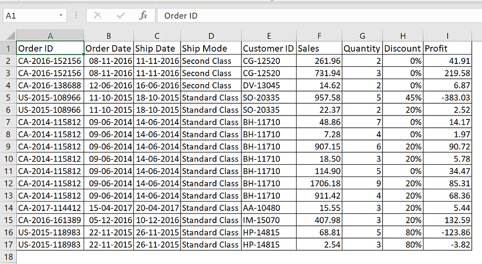
We have sales data, but sequence of columns is not in the desired order.

Our usual process is cut the column and paste in new sheet based on our desired order.

But there is a simple process which can reduce time and errors.

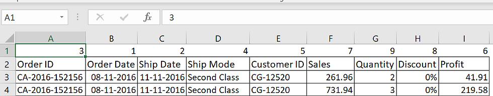
Insert empty row above our data and place order of desired sequence as shown below.

Select entire data from A1:I18,

In menu bar -> Data -> Sort & Filter group -> Sort

In Sort dialog box, click Option as shown below,

Sort options dialog box will open, select 'Sort left to right' radio button and click OK.

In sort by option, select row 1, in Order, select smallest to largest and click OK.

Now we can delete the numbers in row 1. Order of the columns changed based on our input. Simple but powerful.

Trick 2 - Replace Alt + Enter with space:

We have names with line feed or Char (10) in between first name and last name. When we manually enter this data, we use Alt + Enter to move next line within the cell.

Our requirement is to replace the char (10) with space through user interface.

Find and Replace option in excel does that with 100% perfection, but the issue here is to find the line feed. we cannot use Alt + Enter in find box.

To get into Find and Replace dialog box,

In menu bar -> home tab -> Editing group -> Find & select drop down -> Replace.

Or we can simply use the shortcut key Ctrl + H to open Find and Replace dialog box.

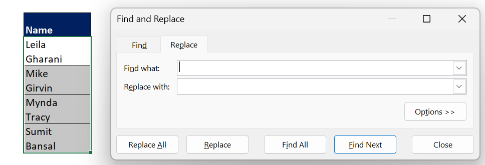
In Find what box, if we type Alt + Enter, excel not able to understand. But instead, type

Ctrl + J short cut key in 'Find what' box, then cursor in that box will change as shown below.

This means, it is in the next line, now in 'Replace with' box press space without any double quotes and click replace all.

Our final output is shown at left side picture. We can use the same shortcut key Ctrl + J in 'text to columns' option to search for line feed delimiter.

Trick 3 - Fill down in Excel:

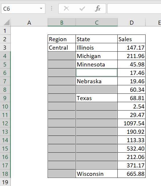
Sometimes we get data with blank cells,

Here in left side picture, you can see that, all the states belong to Central region and so they kept blank after the first occurrence.

This applies for states also.

Wherever blank is there we need to fill down the values in above cell.

To select entire range, follow my steps,

Click B2 cell and press Ctrl + Shift + Right arrow, then press Ctrl + . (Period) to shift the active cell into D2 cell.

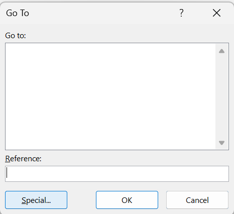
Now press Ctrl + Shift + Down arrow to select entire range. To get active cell into B2 press Ctrl + . (Period) again for 3 times, to open Goto dialog box use shortcut key Ctrl + G or press F5. Click Special as shown below. In Goto special dialog box, select radio button for Blanks and click OK.

You can see that blank cells in our data got selected. Do not disturb anything, just press = and up arrow key and press Ctrl + Enter.

That's it, select entire range, Copy and paste it as values.