Method to create dynamic chart range in Excel - Formula and named range

Today we are going to discuss about, dynamic chart range in excel using formula and named range. Lot to learn, let's dive in.

We will accomplish this in 3 steps.

• Create dynamic range for charts using INDEX function,

• Create named range for this function,

• Use named range in chart axis.

Our data comprises 2 columns, month and sales.

We have clustered column chart to show monthly sales,

Month in category area and sales in values area.

As of now, chart range is not dynamic. If we add data or remove data, chart will not get updated, as shown below.

When we inserted a chart, we fixed the chart range B3:C8, as shown below.

So, when as add or delete our data, chart is not able to make adjustment in size.

To accomplish first step in our task,

We are going to use INDEX function to get dynamic range.

Formula in F4 cell is,

=$B$4:INDEX($B$4:$B$15,COUNTIF($B$4:$B$15,"?*"))

Let me de-construct this into digestible pieces,

Take the INDEX part after colon,

Arguments of INDEX function,

=INDEX(array,row_num,[column_num])

In array argument, we fed the range B4:B15 to accommodate more data,

In row_num argument, we used COUNTIF function.

Argument of this function,

=COUNTIF(range,criteria)

This function helps us to count the number of occurrences of given criteria.

In range argument, we fed the same range B4:B15,

In criteria, we used wildcard characters,

? - represents any one character,

* - represents zero or more characters.

If we feed 'Jan' as our criteria, then this function counts the number of occurrences of 'Jan' in the range B4:B15 and will throw 1 as output.

Here, our criteria are,

the cell value has to have at least one or more character. If so, then add in the count.

This wildcard characters will include only texts and alphanumeric strings.

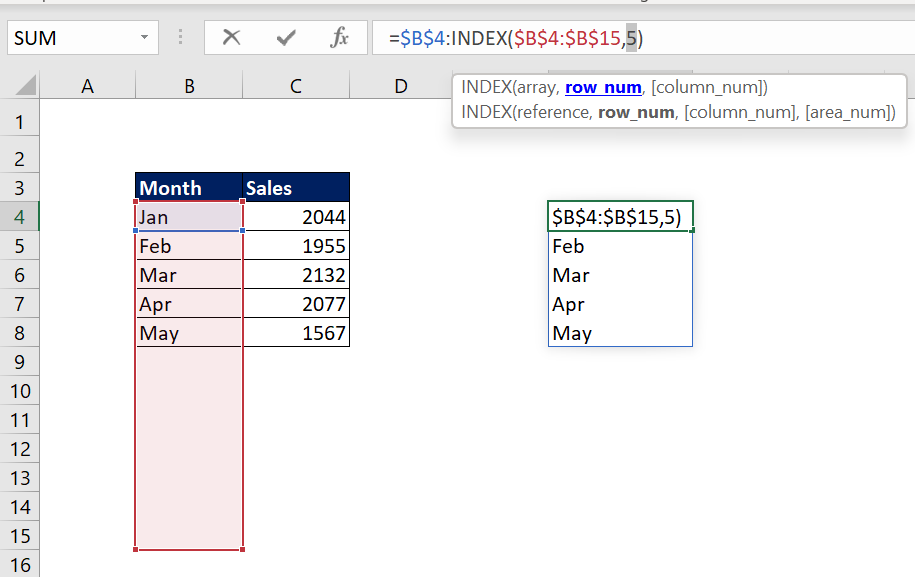
Here, 5 cells are there with characters at least one or more. So, this function throws 5. Then INDEX helps us to get the 5th cell range which is B8.

To know more about output of INDEX function, please visit the below post.

https://www.excel-end.com/post/difference-between-index-and-vlookup-function-advanced-level

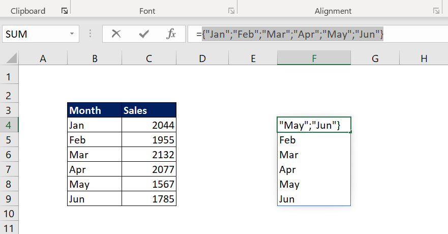
Then the resulting array of $B$4:$B$8 is,

If we add 'Jun' month sales, this function includes 'Jun' in resulting array.

We are going to use this dynamic range for our category axis (X- Axis) in chart.

With bit of tweak in our formula, we are going to get dynamic range for series values (Y-Axis).

For the sake of your learning, I will start this formula from scratch.

Formula in G4 cell is,

=$C$4:INDEX($C$4:$C$15,COUNTIF($B$4:$B$15,"?*"))

COUNTIF part is same as above case, but here, we have added 'Jun' month sales, so this function delivers 6 as output.

We fed C4:C15 range in array argument if INDEX function, so it will deliver C9 cell range.

Then $C$4:$C$9 range will become,

Now, we have dynamic range for both X-axis and Y-axis.

To accomplish our 2nd step, we are going to add these into named ranges.

Named range for X and Y axis:

Copy the formula from F4 cell, then press shortcut key Ctrl + F3 to open 'Name Manager' dialog box. Click 'New' to open 'New Name' dialog box as shown below.

In Name section, we gave 'XAxis' to name our dynamic range and paste the formula in 'Refers to' area and click OK.

In same way, Copy the formula in G4 cell, then create new name 'YAxis" and paste the formula in 'Refers to' area and click OK.

In 'Name Manager' dialog box, select 'YAxis' and click in the formula bar in 'Refers to' as shown below. You can see that excel refers the resulting range of this formula with dotted lines. Now all looks good, we can proceed further.

Formulas in F4 and G4 cell served their purpose, now we can delete them.

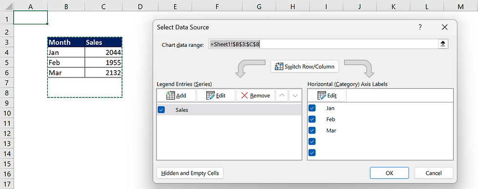
Select the chart, in menu bar, click chart design -> select data.

In select data source dialog box, click 'Edit' button in legend entries (series) area,

Edit series dialog box will open, in series values section, delete everything after "!" sign as sown below.

Press shortcut key F3, to open 'Paste Name' dialog box, select YAxis and Click OK.

Series values in Edit series dialog box will look like below right side picture.

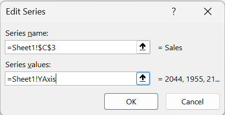
This is the global reference for chart range with name.

='Sheet name' ! 'named range'.

Repeat the same process to edit horizontal category axis label range as shown below.

Now, chart getting updated in dynamic way based on the change in source data.