

Reverse Columns Using the MAP Function in Excel
- V E Meganathan
- Mar 6
- 1 min read
The source data consists of columns labeled Cities1, Cities2, up to Cities5.Each column holds a different number of city names.

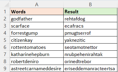
The objective is to reverse the city names within each column.
=LET(a,A2:E19,MAP(a,LAMBDA(x,IFERROR(INDEX(a,ROWS(TOCOL(TAKE(x:E19,,1),3)),COLUMN(x)),""))))
How It Works
LET(a, A2:E19, …) Defines the working range once, making the formula cleaner.
MAP(a, LAMBDA(x, …)) Iterates through each element of the range. x represents the current cell.
TAKE(x:E19,,1) Narrows the focus to the vertical slice of the column that begins at the current cell x and runs down to the bottom of the defined range. By specifying 1 as the column argument, we ensure that only the first column of that slice is returned effectively isolating the portion of the column we want to reverse.
TOCOL(…,3) Converts that slice into a single column vector, ignoring blanks and errors.
ROWS(TOCOL(…)) Counts how many entries are in that slice. This effectively calculates the “reverse position".
INDEX(a, …, COLUMN(x)) Fetches the value from the same column, but from the bottom up.
IFERROR(…, "") Ensures blanks are returned if no value exists.


Comments