Tricks in GROUPBY Function - Excel

Sorting Month Names within the GROUPBY Function in Excel:

The input table includes columns for Month and Sales.

Our objective is to aggregate sales by the month column and arrange the months in chronological order: Jan, Feb, Mar, and so on. 

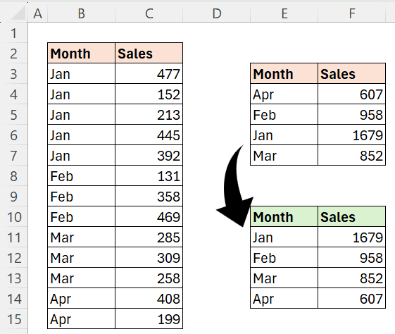
=GROUPBY(B2:B15,C2:C15,SUM,3,0)

This formula will correctly summarize the data but will sort the months alphabetically. 

=LET(m,B2:B15,DROP(GROUPBY(HSTACK(MONTH(m&0),m),C2:C15,SUM,3,0),,1))

This approach summarizes the sales and sorts the months in the correct sequence.

By including the month number as the first column in the row_fields argument, we enable proper sorting of the months. After grouping, the DROP function removes this helper column.

GROUPBY function allows you to access all values within row_fields for each group:

Our objective is to calculate the Percentage of the Grand Total for each region.

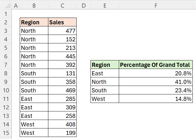
This can be done by simply using the function as shown below:

=GROUPBY(B3:B15,C3:C15,PERCENTOF,0,0) 

However, the LAMBDA function within GROUPBY can handle two variables:

1 -> the values of each group,

2 -> the values of the entire row field, 

Therefore, we can apply the LAMBDA method here:

=GROUPBY(B3:B15,C3:C15,LAMBDA(rows,all,SUM(rows)/SUM(all)),0,0)

This represents the simplest form of LAMBDA with two variables, and this method can also be used for more advanced analysis.

Example of Using the Filter Array Argument in the GROUPBY Function - Excel:

The objective is to calculate the total sales per region, considering only sales values exceeding 250.

=GROUPBY(B3:B15,C3:C15,SUM,0,0,,C3:C15>250)